ผลต่างระหว่างรุ่นของ "Probstat/notes/t-distributions"
Jittat (คุย | มีส่วนร่วม) |
Jittat (คุย | มีส่วนร่วม) |
||
| (ไม่แสดง 3 รุ่นระหว่างกลางโดยผู้ใช้คนเดียวกัน) | |||
| แถว 32: | แถว 32: | ||
<center> | <center> | ||
| − | <math>P\{ -1. | + | <math>P\{ -1.383 < T < 1.383 \} = 0.8</math>, |
</center> | </center> | ||
| แถว 42: | แถว 42: | ||
<math> | <math> | ||
\begin{array}{rcl} | \begin{array}{rcl} | ||
| − | P\{ -1. | + | P\{ -1.383 < \sqrt{n}(\bar{X}-\mu)/S < 1.383 \} |
| − | &=& P\{ -1. | + | &=& P\{ -1.383/\sqrt{n} < (\bar{X}-\mu)/S < 1.383/\sqrt{n} \} \\ |
| − | &=& P\{ -1. | + | &=& P\{ -1.383S/\sqrt{n} < \bar{X}-\mu < 1.383S/\sqrt{n} \} \\ |
&=& 0.8. | &=& 0.8. | ||
\end{array} | \end{array} | ||
| แถว 53: | แถว 53: | ||
<center> | <center> | ||
| − | <math>(100 -1. | + | <math>(100 -1.383\sqrt{5}/\sqrt{10}, 100 + 1.383\sqrt{5}/\sqrt{10}) = (99.022, 100.978).</math> |
</center> | </center> | ||
| แถว 105: | แถว 105: | ||
and note that the form of the quantity matches the definition of the ''t''-distributed random variable where <math>Z=\frac{\bar{X}-\mu}{\sigma/\sqrt{n}}</math> and <math>X = \frac{(n-1)S^2}{\sigma^2}</math>. | and note that the form of the quantity matches the definition of the ''t''-distributed random variable where <math>Z=\frac{\bar{X}-\mu}{\sigma/\sqrt{n}}</math> and <math>X = \frac{(n-1)S^2}{\sigma^2}</math>. | ||
| + | |||
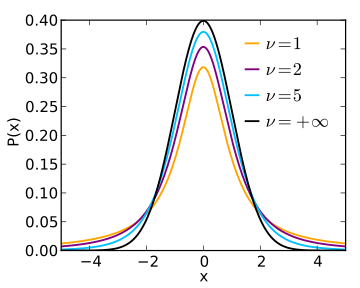
| + | The ''t''-distribution is a flatten-out version of the normal distribution (see pdf below). It gets closer and closer to the normal distribution as the degrees of freedom increase. See [http://en.wikipedia.org/wiki/Student%27s_t-distribution wikipedia's article] for more graphs and information. | ||
| + | |||
| + | [[Image:Student t pdf.svg]] | ||
| + | (Image from [http://en.wikipedia.org/wiki/File:Student_t_pdf.svg]) | ||
| + | |||
| + | == Links == | ||
| + | * [http://en.wikipedia.org/wiki/Student%27s_t-distribution wikipedia article] | ||
รุ่นแก้ไขปัจจุบันเมื่อ 10:00, 6 ธันวาคม 2557
- This is part of probstat.
In many applications including computing confidence intervals and also hypothesis testing, we need to know the distribution of the sample mean. Let be a sample mean of a normal population computed from a sample of size . If the variance of the population is known, we have that
However, in most cases, we do not know and we only have the sample variance
.
Therefore, we would like to use the sample standard deviation instead of the real standard deviation . We hope that
will be close to normal. This is indeed true. Although is not normal, it is t-distributed with degrees of freedom. (See definition below.) Therefore, we can use the table for the t-distribution to compute probabilities for various events related to this statistic. Note that it is slightly harder to use than the standard normal table, because there are two parameters, i.e., the degrees of freedom and the level of confidence that you want.
We will show example usages for the t-distributions and then discuss the mechanics behind this usage of the t-distribution.
EX1: We take a sample of size 10 and calculate the sample mean and the sample variance . Find the confidence interval with 80% confidence level.
Solution: Since the sample size is 10, the degrees of freedom to use is 9. We look at the t-table and find out that
,
where is a t-distributed random variable with 9 degrees of freedom.
Since , we have that
If we put in the actual values of and we have that the confidence interval with 80% confidence level is
Comparison with the case where is known. As a comparison, suppose that the real variance is actually 5. Using the standard normal table, our confidence interval will be smaller. That is, we have that
Plugging in the values of and we have that the confidence interval with 80% confidence level is
which is slightly smaller the previous interval.
Student's t-Distribution
Note that our goal
Let's recall two important facts about sample means and sample variances. First, and further more, and are independent. These imply that the above quantity is a quotient of a unit normal random variable and a square root of a chi-squared random variable. This is exactly what a t-distributed random variable is.
Definition: If is a unit normal random variable and is a chi-squared with degrees of freedom, such that and are independent, we call a random variable
a t-distributed random variable with degrees of freedom.
To see that is t-distributed with degrees of freedom, we calculate
and note that the form of the quantity matches the definition of the t-distributed random variable where and .
The t-distribution is a flatten-out version of the normal distribution (see pdf below). It gets closer and closer to the normal distribution as the degrees of freedom increase. See wikipedia's article for more graphs and information.
 (Image from [1])


